Single pulse analysis

Kookaburra provides a command-line tool for fitting single pulses. To get help with this, run

$ kb_single_pulse --help

This takes a single positional argument, the data to analyse, and a number of optional arguments related to the choice of model to fit and priors. We provide a quick-start example on simulated data below.

Quick start

To demonstrate the basic input and output, we will create simulated data from a pulsar (flux as a function of time) and analyse it. First, we run the script make_fake_data.py available in the examples directory. Here are the contents:

""" Script to generate a data file with a single simulated pulse

Usage:

    $ python make_fake_data.py

This will generate a file fake_data.txt, a comma-separated file of the time
vs. flux for the simulated signal. The simulated signal contains a simple
first-order polynomial base flux and a three-component shapelet pulse.

"""
import numpy as np
import pandas as pd

import kookaburra as kb

# Injection parameters
pulse_injection_parameters = dict(
    C0=0.6, C1=0.1, C2=0.2, beta=1e-3, toa=0.005,  # Parameters for the shapelets
    B0=1, B1=-20  # Parameters for the polynomial base-flux
)


# Instantiate a flux model: a sum of the shaplet and polynomial flux classes
flux_model = kb.flux.ShapeletFlux(3) + kb.flux.PolynomialFlux(2)

# Generate fake data using the instantiated flux model and injection parameters
N = 1000
time = np.linspace(0, 2 * pulse_injection_parameters["toa"], N)
flux = flux_model(time, **pulse_injection_parameters)

# Add Gaussian noise
sigma = 2e-2
flux += np.random.normal(0, sigma, N)

# Write the data to a text file
df = pd.DataFrame(dict(time=time, flux=flux, pulse_number=0))
filename = "fake_data.txt"
df.to_csv(filename, index=False)

This will create a file fake_data.txt.

Now we can run kb_single_pulse on this data file.

$ kb_single_pulse fake_data.txt -p 0 -s 5 -b 2 --plot-fit

The flag -p sets the pulse number to extract from the data file. For this example simulated data only a pulse 0 exists, but in general a data file could contain many pulses. The flag -s sets the number of shapelets to use in the fit. When simulating the data, the model had 3 shapelets. Here, we set a maximum number of 5. The flag -b sets the order of the base polynomial. Here we chose a first order polynomial. If you do not need to remove a baseline, set -b 0. Finally, we include flags to plot the data (this will be done before the main analysis begins) and the fit to the data.

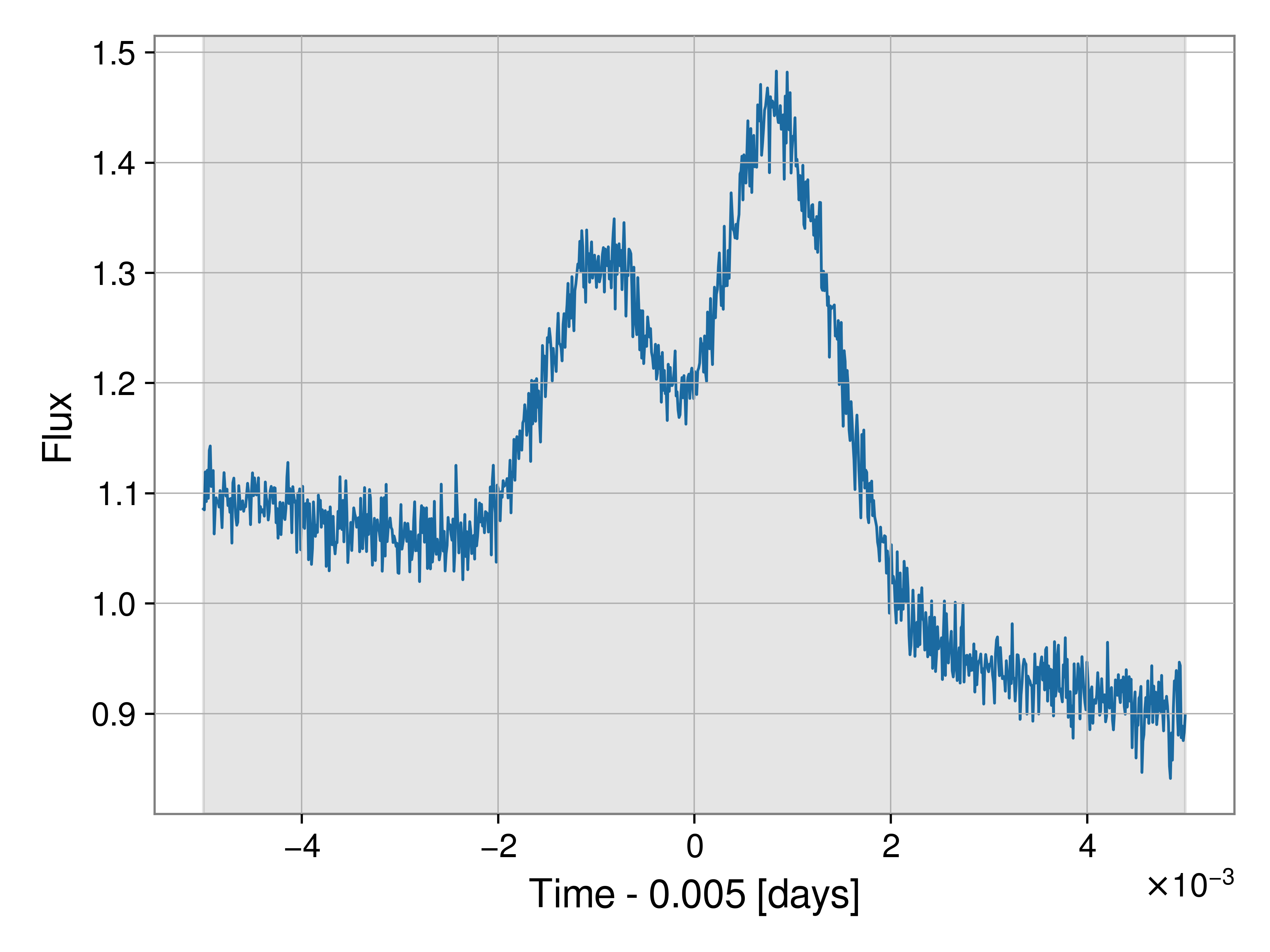
Here is the figure of the data itself, the gray band indicates the prior range (in this case, the whole data span).

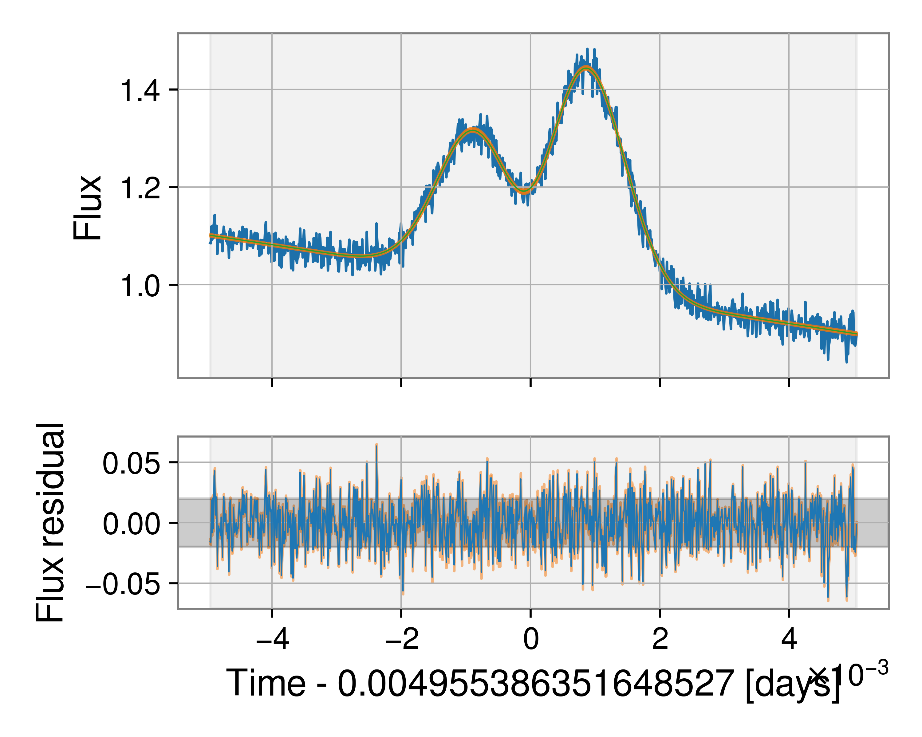
Here is the figure of the fit to the data. The green line indicates the maximum likelihood fit, while the orange band indicates the 90% model uncertainty around this fit. The lower plot illustrates the residual after subtracting the maximum likelihood model while the orange shaded region again indicates the uncertainty in the residual.

The code outputs all results to outdir/ by default (this can be changed with a command-line argument). The result itself is the .json file, this is a bilby json file, but with extra information stored such as the residual.